 Onsieve capabilities
From plant data to forecasts and operator software
Onsieve forecasts how an industrial plant will perform and, when required, provides the operator software to run it against that forecast: every hour tracked, every deviation flagged and explained. Shown here on a seawater reverse osmosis plant.
One model, from forecasting analysis to daily operation
Shown on a seawater reverse osmosis plant: the same approach applies to any engineered process with a data historian.
Learn the plant and forecast it
Your historian data · hourly · all signals
Onsieve reads every flow, pressure, quality and energy signal together and trains machine learning and neural network models of how the plant produces, keeping whichever generalises best to data it never saw. It is proven against a classic forecast, then projects the year ahead.
Deliverable: validated forecast + report
Package the plant’s expected behaviour
Hourly outlook · calibrated 5–95 % band
The forecast and its uncertainty become the plant’s procedural model: what the plant should do, hour by hour, and how far it may honestly stray before something is wrong.
Deliverable: a procedural model of the plant
Run the plant against its procedural model
Onsight Operator · for the operations team
When required, Onsieve provides the software the operations team uses every day: upload plant data, see whether the plant is on track, get deviations flagged and explained, retrain the outlook in one click.
Deliverable: operator software, configured for the plant
The analysis stands on its own; the operator software reuses the same model, with no second project.
The showcase: a seawater reverse osmosis section
Ultrafiltered seawater in, low-salinity water out. Split-partial 1st pass with energy recovery, polishing 2nd pass. Forecast target: the product flow to the blending tank, ≈ 5,600 m³/h.
One year of plant memory, hour by hour
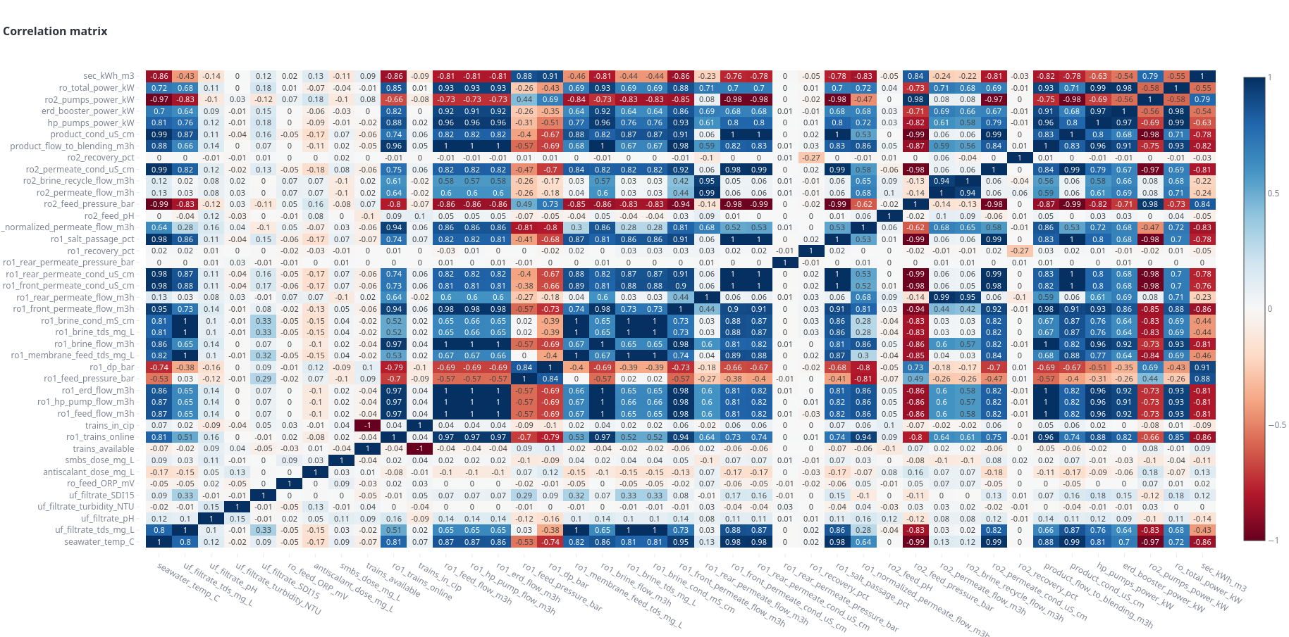
What moves together: 41 signals, one matrix
Forecasting analysis
The first Onsieve deliverable: a model that reads the plant, proven against a classic time-series forecast.
A procedural model is grown from data, not hand-tuned
This is what makes the next two slides possible: the model is not fitted to a calendar, it is trained on the plant itself.
Every signal, hour by hour
All plant flows, pressures, qualities, trains and chemistry from the historian: 41 signals × 8,760 hours in this showcase, nothing invented.
What actually drives the target
The signals most correlated with the target are picked automatically from the data itself — the hydraulic state of the 1st pass, in this showcase.
Train and compare
Machine learning and neural network models are trained on that data; the one that generalises best is kept, not the one that fits the training data hardest.
Proven, not assumed
Tested on weeks the model never saw in training, with separate 5 % / 95 % models so the uncertainty band is calibrated, not guessed.
The deliverable
The validated model, its calibrated band and its input relationships become the plant’s procedural model — what the plant should do, hour by hour.
No equation is written by hand: the machine learning and neural network models learn the plant’s own behaviour directly from its data, which is exactly why the forecast stays accurate when the plant does something a hand-written formula never anticipated.
Fitting a curve, or learning the plant
Both models were trained on the same data and tested on the same ten weeks.
Extends the curve of the past
- Sees only the target and the calendar: trend, weekly and yearly seasonality
- A step change, such as a train stopping, is invisible until it has happened, and then it is treated as an outlier
- Its uncertainty band is drawn from the past curve, so it is overconfident when the plant changes mode
- Says nothing about why a value is high or low
Good for smooth, seasonal series with no physical drivers.
Learns how the plant produces water
- Trains machine learning and neural network models on the plant signals that drive the target: flows, pressures, trains, quality
- When the plant changes mode, the inputs change and the forecast follows immediately
- Separate 5 % and 95 % models give a band that holds its promise: 92.9 % of the test values fall inside the 90 % band
- Every prediction can be decomposed into its inputs, which later explains deviations
Built for engineered systems, where physics and operating decisions drive the numbers.
Ten weeks the model never saw
Not in the same league
90 % band: does it hold its promise?
Share of the measured test values inside each model’s 90 % band. Target: 90 %.
One year ahead, 8,760 hours
Operator software
Optional, after the analysis: Onsieve provides Onsight Operator, the software the operations team uses to manage the plant against its procedural model.
What the operator software does with every upload
Supplied and configured by Onsieve, used by the operations team: no data scientist in the loop.
The model
Onsieve loads the forecast and its 5 % / 95 % models into Onsight Operator as one model file.
Daily plant data
CSV or Excel, any number of rows, upserted by timestamp. Here: 7,224 rows, 296,184 cells, 0 invalid.
Plant vs forecast
Each hour is checked against the band the model committed to, not an invented threshold.
Events
Consecutive hours outside the band are grouped into events, with peak and mean deviation.
Candidate causes
Every signal is compared with its own history, checked for timing and correlation with the deviation.
New outlook
One click refits the model on history + uploads and issues a fresh forecast from today.
Evidence about the plant and explanation of the model are kept apart: the operator sees what the plant did, not what the algorithm prefers.
Ten months on track, then the plant leaves the forecast
Telling noise from a real change
Isolated blips
Single hours just outside the band, scattered from June to October. Nothing persistent.
On trackA persistent deviation
Four hours in five outside the band, almost all of them above the forecast: +4.3 % of the week’s water.
Persistent deviationThe deviation travels with the first-pass flows
Evidence, not a manufactured root cause
| Candidate | Link on record | Actual (mean) | Expected | r with residual |
|---|---|---|---|---|
| Front permeate flow | model input | 3,401.8 | 3,398.3 | 0.99 |
| 1st pass feed flow | model input | 13,080.6 | 13,067.3 | 0.99 |
| HP pump flow | model input | 5,907.7 | 5,901.7 | 0.99 |
| Brine flow | model input | 7,259.3 | 7,251.9 | 0.99 |
| ERI flow | model input | 7,260.0 | 7,252.7 | 0.99 |
| 2nd pass permeate flow | not documented | 2,128.5 | 2,126.3 | 0.99 |
| Specific energy | not documented | 2.498 | 2.502 | −0.81 |
| Seawater temperature | not documented | 26.95 | 26.98 | −0.62 |
Onsieve adds the plant’s physics: a hint becomes a finding
| Engineering check (from the scheme) | What it would catch |
|---|---|
| product = front permeate + 2nd pass permeate | Meter drift on the blending line |
| feed = HP pump flow + ERI flow | Flow meter inconsistency within a train |
| HP power ∝ flow × (feed pressure − suction) | Power or flow meters that disagree |
| trains online, CIP → operating state | Separate a decision from an anomaly |
| feed pressure ≤ 76 bar · 2nd pass ≤ 18 bar | Design envelope, before the trip |
Explaining the model, separately from the plant
What the model leans on
Mean |contribution| over the training data, m³/h
| Input | Assumed | Measured | Δ | Model-attributed Δ |
|---|---|---|---|---|
| Front permeate flow | 3,398.3 | 3,401.8 | +3.5 | +0.96 |
| HP pump flow | 5,901.7 | 5,907.7 | +6.0 | +0.46 |
| 1st pass feed flow | 13,067.3 | 13,080.6 | +13.3 | +0.37 |
| Brine flow | 7,251.9 | 7,259.3 | +7.4 | +0.25 |
| ERI flow | 7,252.7 | 7,260.0 | +7.4 | +0.09 |
Not just a better forecast: a forecast the plant can run on
A forecast is only as useful as what the operations team can do with it.
| Simple forecast (Prophet) | Onsieve: forecasting + operator software | |
|---|---|---|
| What it reads | Target + calendar | All plant signals: flows, pressures, trains, quality |
| Mode change (8 → 7 trains) | Misses it: 14.6 % error after the step | Follows it: 0.43 % over the whole test |
| Mean error on unseen weeks | 631 m³/h | 22.5 m³/h |
| 90 % band holds? | No: 5.3 % coverage | Yes: 92.9 % coverage |
| Usable as an alarm limit | No: would alarm 95 % of the time | Yes: 18 flagged hours in ten months |
| Says why a value deviates | No | Ranks candidate signals by evidence |
| Keeps learning | Refit by an analyst | One-click retrain on every upload |
Missing or faulty data? Rebuilt with you, step by step
This showcase dataset was complete (0 invalid of 296,184 uploaded cells); most plant historians are not. The same method applies either way.
Map every gap
Each signal is scanned for gaps, frozen values, spikes, drifts and unit errors, hour by hour, and shown on a data-quality map.
Set the rules with you
With the plant team: which sensors to trust, which periods are shutdowns or tests, what may be filled and what must stay empty.
Reconstruct
Gaps are rebuilt from the plant balances (flows, recovery, pumps) and from correlated signals with machine learning and neural networks.
Test the reconstruction
Known data are hidden on purpose and rebuilt: the reconstruction error is measured before any value is accepted.
Approve, period by period
The client reviews each reconstructed period on the charts and approves it, or sends it back with plant knowledge.
Flag, never hide
Every rebuilt value stays tagged in the dataset and in the operator software; forecasts state how much of their history was reconstructed.
Real historians have holes. Onsieve does not wait for perfect data: it rebuilds it transparently, with the people who know the plant.
What Onsieve delivers
Start with the analysis; add the operator software when the plant is ready for it.
A validated forecast of your plant
- Data audit and, where needed, reconstruction of gaps and faulty sensors, agreed step by step
- Machine learning and neural network models for the targets that matter: production, quality, energy
- Accuracy measured on data the model never saw, and reported before delivery
- Hour-by-hour outlook with a calibrated 5–95 % band
- Interactive report and presentation of the results
Stands on its own: production planning, budgets, maintenance windows.
The plant’s procedural model in the operators’ hands
- Procedural model deployed from the same models: no second project, no new pipeline
- Daily upload (CSV or Excel), hourly tracking against the procedural model’s band
- Alarms as events, with candidate causes ranked by evidence
- Operating states and engineering checks configured by Onsieve for the plant
- One-click retrain, saved sessions, CSV / JSON export of every diagnosis
Turns the analysis into a daily tool to manage and supervise the plant.
Solid forecasts and a clear view of the plant, guaranteed by validation
Results proven before delivery. Every model is tested on data it never saw. Accuracy and band coverage are measured and reported up front: here 0.43 % error and 92.9 % of hours inside the 90 % band. You sign off on figures, not promises.
Machine learning and neural networks. Onsieve builds and compares machine learning and neural network models for each target; the one that performs best on unseen data is the one delivered.
Forecasts that hold when the plant changes. Because the models read the plant signals, they follow operating decisions: 28× lower error than Prophet, through a change from 8 to 7 trains.
Tools to understand the plant. Correlations, each signal against its own history, events, ranked causes, engineering checks and model transparency: the team sees what changed and why.
Imperfect data is not a blocker. Gaps and faulty sensors are reconstructed step by step with the client, tested and flagged, so the analysis can start from the historian you already have.